Joana da Matta
Cohere Labs Community, Unicamp
Joana is a MSc Student in Computer Science researching fairness and interpretability in machine learning, and co-leads the ML Understanding program at the Cohere Labs Community.
A community study of whether stereotype-congruent concepts surface in the internal workspace of Qwen3.5, where they appear, what shapes them, and whether they actually drive the model's answers.
TL;DR
- Yes, sometimes. In Qwen3.5-4B, stereotype-congruent tokens surface in the Jacobian-lens workspace even when the output never states them, and even when the context has already settled the answer.
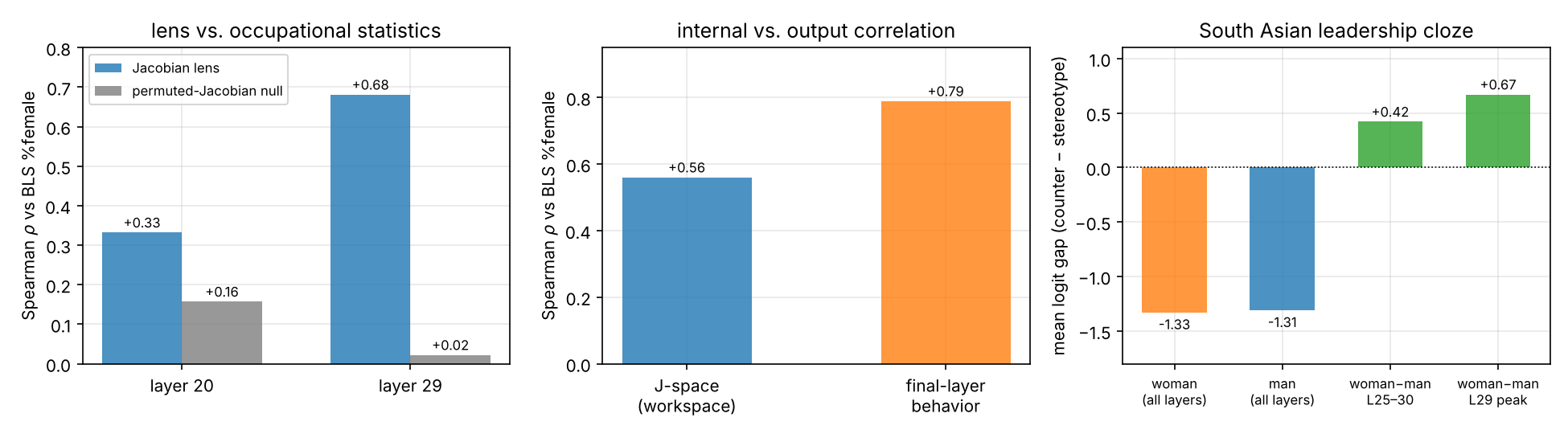
- Gender is the clearest case. The lens’s gendered preference for each occupation tracks US labor statistics (Spearman ρ rises from +0.332 at layer 20 to +0.681 at layer 29), while a permuted-Jacobian null stays flat.
- Beyond gender, the evidence is fragile. On the balanced BBQ benchmark we found no significant aggregate signal. Baseline group preferences explain 63–98% of the variance, and the choice of descriptor word (“weak” vs. “submissive”) can move the readout more than the choice of group.
- There is no single “bias layer.” Correlations peak around layers 23–25, layer 27 makes both answers accessible at once, and steering works best at layers 29–30.
- The lens is a causal handle, but a blunt one. Swapping lens directions changes answers, yet most of the effect comes from ablating the answer the model was already giving. At large intervention strengths (α ≥ 3) the output falls apart.
- The method lesson: a lens readout must be treated as evidence, rather than proof. We recommend triangulating across lenses, controls and datasets.
| Research question | Short answer | Section |
|---|---|---|
| RQ1. Do stereotype-congruent tokens surface in the lens? | Yes, most clearly for gender and occupations. Aggregate significance on balanced datasets is contingent on measurement choices. | RQ1 |
| RQ2. Where in the network does the signal show up? | Mostly late-intermediate layers (≈23–30), but the band depends on axis, metric and prompt format. | RQ2 |
| RQ3. How do context, wording, format and pressure reshape it? | A lot. Descriptor wording, prompt format and pressure often matter more than group identity. | RQ3 |
| RQ4. Does the signal causally drive the answer? | Partly. Lens directions are a handle on the committed answer, but swaps add little beyond ablation. | RQ4 |
Most bias benchmarks, such as BBQ
This post summarizes a multi-week Cohere Labs Community project that tries to look at that process. We use the Jacobian lens (J-lens) to ask whether stereotype-related content can be detected inside a model, where it appears, how it changes with context, and whether it actually drives the answer. All code and materials are in the group repository.
In July 2026, Anthropic’s interpretability team published Verbalizable Representations Form a Global Workspace in Language Models
To explore this, they introduce the J-lens and the related J-space, and test the workspace-like properties of that space with causal interventions, not only correlations. The tool is released as the open-source jacobian-lens library. We use it with a pre-fitted lens on Qwen3.5-4B.
How the lens works. A model produces its answer one token at a time, but most of the computation happens in the residual stream of the hidden layers, where nothing is printed. The classic logit lens reads this stream by applying the unembedding matrix directly at an intermediate layer, which gets unreliable in early layers because the stream does not use the same coordinates at every layer.
The J-lens instead describes an activation through its first-order causal effect on the model’s outputs. Let
The result is a score for every vocabulary token: the words the activation is, on average across contexts, disposed to make the model say. The logit lens is the special case
This lets us see concepts that never appear in the input or the output. In the paper’s example, the prompt “The number of legs on the animal that spins webs is” surfaces spider in intermediate layers, though the word is in neither the prompt nor the answer. This means we can look for the stereotype the model considered but did not say.
Caveat. The authors describe the J-lens as an imperfect, approximate tool, and its readouts are noisy in roughly the first third of the model. We take this into consideration throughout the experiment.
Models and lenses. Most experiments use Qwen3.5-4B with the released qwen-n1000 J-lens. A few smaller checks use Qwen3.5-0.8B and we say so where they appear. We also built a second lens, the template lens, to fix a coverage gap. The J-lens is undefined whenever the two answers in a BBQ item share a first token (for example, “grandfather” and “grandson” both start with “grand”), which drops its usable coverage to as low as 19 of 40 quads in some categories. The template lens is made of 833 phrase-level vectors fit from passages generated by Qwen-3.6-27B, and it scores all 40 quads by comparing answers at the first word where they actually differ.
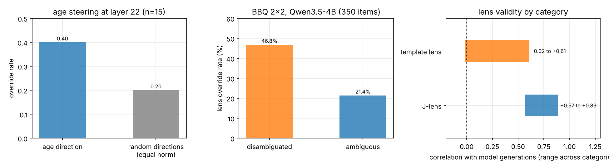
Both lenses pass a basic validity check: on disambiguated items their readouts lean toward whichever answer the text supports, in all 11 BBQ categories, while multiple-choice accuracy on those items ranges from 0.79 to 0.96. They differ in reliability. The J-lens readout correlates with what the model actually generates far more consistently (0.57 to 0.89 across categories) than the template lens does (−0.02 to 0.61). The two are complementary, not interchangeable.
Data. BBQ
Reading the numbers. Several layer bands were chosen after looking at results, and some tests are small. We flag these as exploratory throughout. Treat them as hypotheses for preregistered follow-up.
We first asked whether stereotype-congruent concepts become readable in intermediate and late representations even when the final output does not state them.
Take a BBQ item that asks whether a man or a woman is the secretary, where the context gives no way to decide. Across layers 14–31, the answer-letter token for the woman appeared six times in the lens readout, and the man’s once. The lean persists when the context settles the question. In an item stating that the boy is bad at math, the letter for “girl” still showed up three times in the workspace, against five for the correct answer. The model answers correctly, yet the stereotype-congruent option stays readable internally.
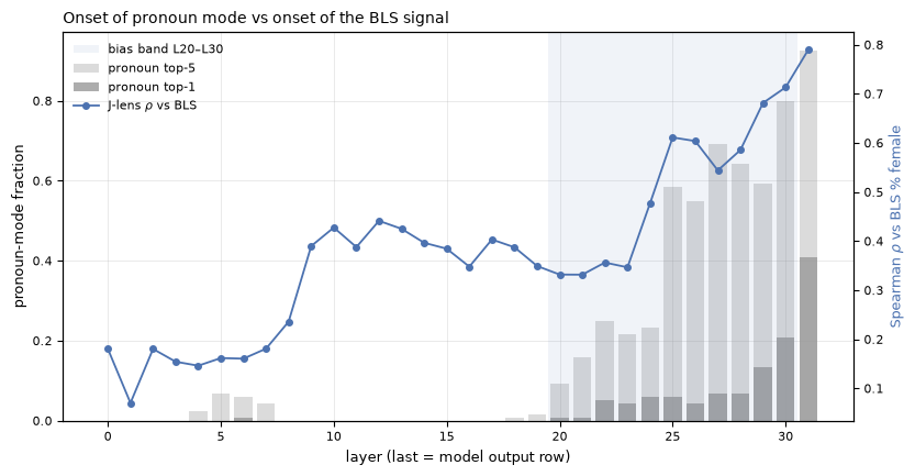
Hand-picked examples can mislead, so we aggregated. Our most robust finding compares the lens’s gendered preference for each occupation with BLS data. Spearman’s ρ rises from +0.332 at layer 20 to +0.681 at layer 29 (p < 0.001), tracking the point where the pronoun becomes the top-ranked token (around layer 28). To check that this reflects learned structure and not an artifact of projecting through any matrix of that size, we built a permuted-Jacobian null matched in norm and spectrum. Its correlation stays flat and non-significant (+0.157 down to +0.022, all p > 0.22). The J-lens also surfaces the association about six layers earlier than the standard logit lens, which reads nothing at layers 20–23.
One result surprised us. Final-layer behavior correlates with occupational statistics more strongly (ρ = +0.789) than the intermediate workspace does (ρ = +0.560). This cuts against the common assumption that intermediate layers hide a stronger bias than the model expresses. Here, the internal signal looks like an earlier, noisier, attenuated version of the bias in behavior.
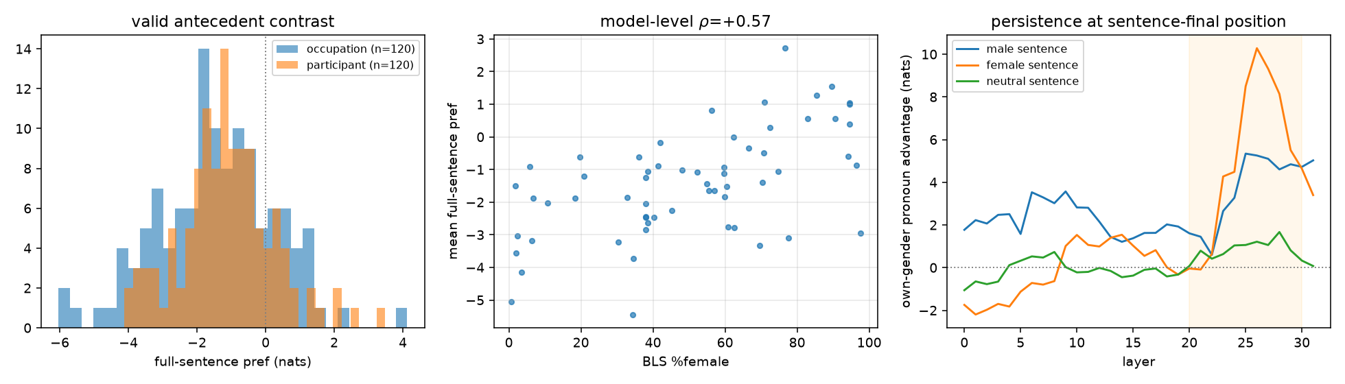
A Winogender follow-up points the same way, though less firmly. Scoring full sentences (which keeps the suffix that identifies the pronoun’s antecedent) over 120 matched pairs, the mean female-minus-male log-likelihood was −1.418 nats for occupation antecedents and −1.103 for participant antecedents. The paired difference of −0.314 nats (95% CI [−0.679, +0.036], Wilcoxon p = 0.069) leans male for occupations, but the interval includes zero, so it is suggestive, not conclusive.
Intersectionality. Adding racial and ethnic descriptors to the “bad at math” item left stereotype-congruent tokens ahead in most variants, even though the context says the boy struggles. But placing “Latino” or “Indian” before “girl” flipped the balance toward counter-stereotype tokens, and “boy” surfaced correctly at layer 31. In the secretary item the descriptors added variation, and the effect vanished once the answer options were removed from the prompt.
In a second analysis, eight English workplace-leadership cloze prompts compared a South Asian woman with a South Asian man (248 prompt-layer observations). The lens ranked the counter-stereotype descriptor above the stereotype one for both (mean logit gap −1.32; −1.33 for the woman, −1.31 for the man). The woman-minus-man difference sits near zero through layer 9, dips slightly in layers 10–19, and turns positive in layers 25–30 (mean +0.42, peaking at +0.67 at layer 29), where the lens agrees most with the model’s output. In short, a gendered asymmetry can survive in intersectional settings, concentrated in late layers, but an ethnic descriptor can also erase or reverse it. Single-axis readings should not be assumed to carry over.
Religion was the strongest candidate outside gender. A raw lens delta mixes a baseline preference for one group’s term regardless of the question (a group prior) with a polarity-dependent preference that actually tracks the stereotype (a bias term). Decomposing ambiguous BBQ items this way, the group prior explains 63–98% of between-item variance across categories, with gender identity highest (0.98 for the J-lens). Religion has the lowest group-prior share (0.63), and the template lens also tracks the model’s generations well there. That makes it the best candidate for a genuine stereotype signal, but only a candidate: religion’s readout also shifted substantially with question polarity, and some of that may reflect the target’s semantic role, not a stable stereotype.
Age was harder. On 40 BBQ Age items at layer 30, ambiguous items were dominated by hedges such as “unclear” and “neither.” Identity terms appeared in the top 20 for 23 of 40 items (57.5%), but stereotype and counter-stereotype terms usually appeared together. Only the disambiguated/negative cell clearly favored the stereotype (mean rank gap +269, median +110.5), and with ten items per cell and a few outliers that could easily be noise. Steering tells a similar story: a difference-of-means age direction at layer 8 turned a hedged answer into a confident counter-stereotype one on one item, but across 15 items random directions of equal norm matched or beat it at layers 8 and 15. Only at layer 22 did it beat every random control (override rate 0.40 vs. 0.20). A single striking example, without random-direction controls, was weak evidence.
We consistently found stereotype-associated tokens in individual prompts, but not always a statistically significant aggregate. In balanced datasets, each group appears equally often in stereotyped and non-stereotyped roles, so effects partly cancel across prompts. A full BBQ 2×2 on Qwen3.5-4B (350 items, 7 categories, all layers) found no aggregate signal at the answer position: the pooled layer-23 median gap on ambiguous items was −64 with 46% positive, and the lens override rate ran opposite to behavior (46.8% disambiguated vs. 21.4% ambiguous). The gaps live in the far tail: the lens puts the stereotype word at median rank around 8,000 of 248k, where the model’s own readout puts it near 111.
Several measurement obstacles make this worse:
There is no single answer, and the layer you find depends on what you measure.
Correlation peaks mid-to-late. In one BBQ and Winogender analysis, balanced gender preference peaked at 0.588 in layers 23–25 (a score where 0.5 means no signal). The BLS correlation rises through layer 29. Pronoun accessibility changes sharply near layer 28, where the pronoun’s rank moves from 233 at layer 0 to 1, and its emergence tracks the occupational correlation profile (rs = +0.821).
Layer 27 exposes both answers. Across seven BBQ datasets, the strongest transition under the answer-text prompt (P2) occurs from layer 26 to 27, where bias and non-bias targets both move toward the top of the vocabulary (cross-dataset mean changes of −1.254 and −1.220). It appears in all seven datasets and under P3 as well.
| Dataset | Bias target | Non-bias target |
|---|---|---|
| Age | −0.869 | −0.801 |
| Physical appearance | −1.262 | −1.213 |
| Religion | −1.396 | −1.369 |
| Disability status | −0.831 | −0.810 |
| Nationality | −1.228 | −1.227 |
| Sexual orientation | −1.684 | −1.657 |
| Socioeconomic status | −1.505 | −1.461 |
Change in target accessibility from layer 26 to 27 (negative means closer to the top of the vocabulary).
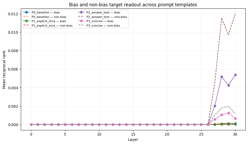
Because both alternatives become accessible together, layer 27 is better read as a task-relevant semantic workspace than as a “stereotype layer.” Bias, where present, is a relative imbalance between jointly accessible targets.
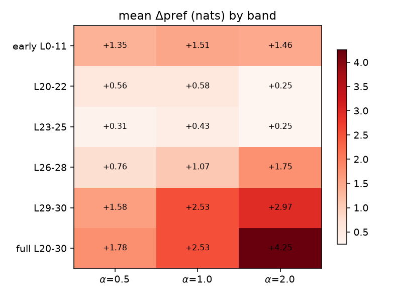
Correlation is not causal leverage. Correlational readouts peak around layers 23–25, but sub-band steering puts the strongest causal leverage later. Intervening only at layers 29–30 reproduced the full eleven-layer steering effect (+2.53 nats), while steering layers 20–25 had little effect (+0.43 to +0.58 nats; 15–20% answer flips). Counterfactual patching, which writes the matched disambiguated residual into an ambiguous prompt, raised evidence-supported answers from under 10% in the earliest layers to about 63% by the low twenties, 71% at layer 27 and 76% at layer 31. The template lens stabilized around layer 23, although patching had already shifted half the prompts by layer 19. So the lens is a delayed correlate of the decision, not a live trace of it.
Early structure can reverse. For South Asian workplace prompts, the English woman-minus-man gap was near zero in layers 0–9 and positive in layers 25–30. Urdu prompts looked different: the woman answer led at layers 0–2 (+2.92 at layer 0), then the preference reversed at layer 3 and stayed negative through layer 30. Early signals can change direction instead of growing into the later English pattern. Age results resist localization altogether: across 40 prompts on Qwen3.5-0.8B, rank gaps varied by item and layer, formatting tokens often outranked both targets, and the largest gap was selected after scanning layers, so we treat them as descriptive only.
Late layers can undo early signals. One multi-band ablation found no output change from layers 0–20, with steerability concentrated in layers 22–30. In the patching curve, the largest single jump (23% to 41%) came at layer 17, a linear-attention layer, in a model that alternates attention types every four layers. Long-range mixing is a possible explanation, but this is preliminary.
Taken together, the evidence supports a late-intermediate workspace for several 4B signals, not one universal localization. The apparent band depends on axis, read position, prompt format and metric. Because several band edges were chosen after inspecting results, treat them as hypotheses, not architectural boundaries.
If the signal were a stable property of the model, it should survive reasonable changes to the prompt. It mostly does not.
Wording and framing beat group identity. We scored four English workplace scenarios, each with its own descriptor pair, for a South Asian woman and man (logit gap averaged over 31 layers). The descriptor pair set the sign of the gap for both groups. “Submissive/assertive” and “timid/confident” favored the counter-stereotype word (about −4.2 and −2.9 for the woman, −3.9 and −2.4 for the man), while “indecisive/decisive” and “weak/strong” leaned toward the stereotype word (+0.34 and +1.48 for the woman, +0.32 and +0.76 for the man). The woman-minus-man difference was small and changed direction across scenarios (−0.24, −0.55, +0.02, +0.72). Each scenario had only one descriptor pair, so wording and framing are confounded, and separating them would need several pairs per scenario. Three Urdu prompts showed a layer-dependent reversal (woman favored in layers 0–2, man from layer 3), but with n = 3 that is only suggestive.
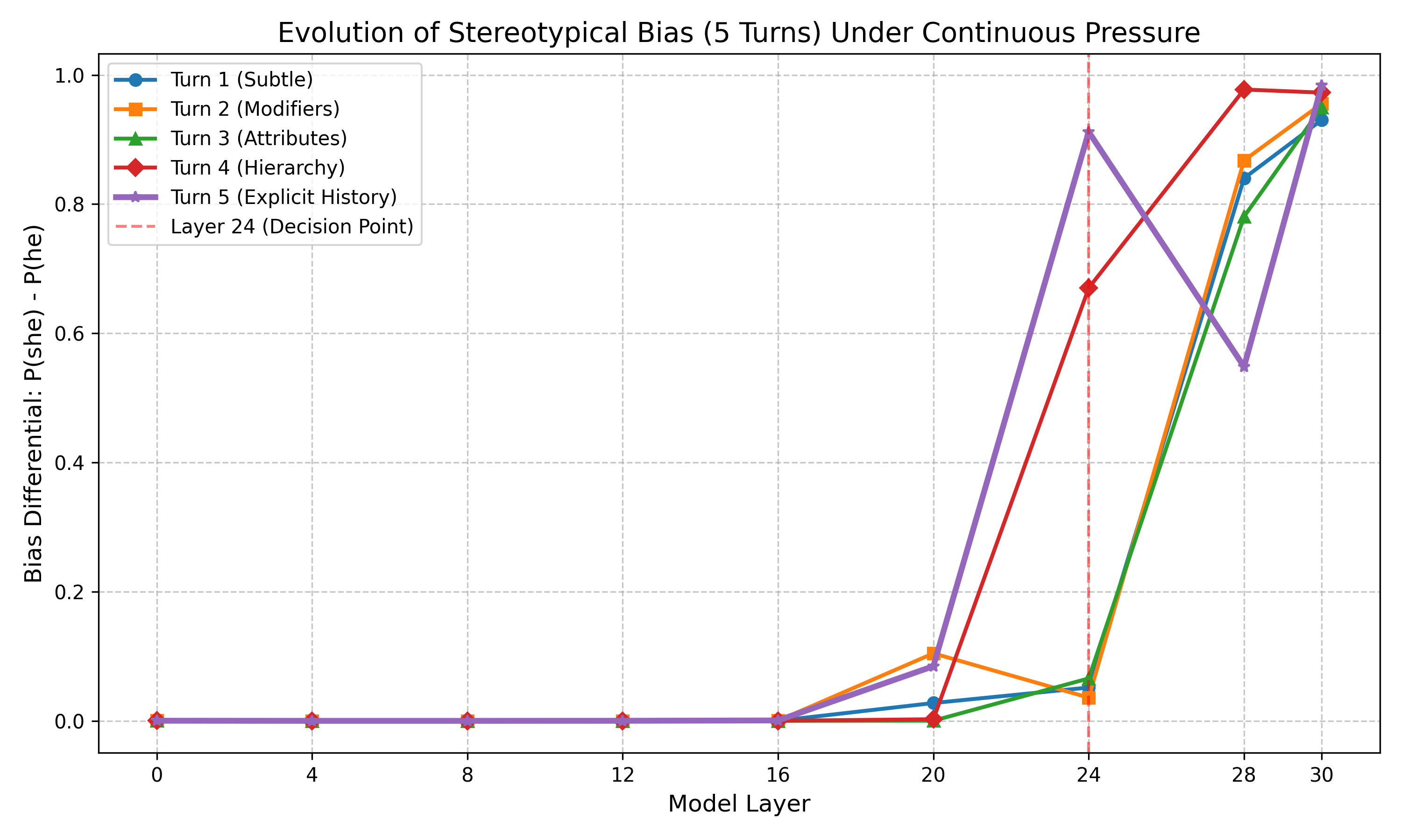
Pressure moves the commitment layer. In a multi-turn adversarial-pressure sequence on Qwen3.5-4B, the layer where P(she) first exceeds 80% moved earlier, from layer 28 to layer 24. Concretely, P(she) was 84.1% at layer 28 in the neutral prompt, 81.0% at layer 24 under explicit pressure, and reached 97.9% at layer 28. This is a condition-specific trajectory, not a universal layer boundary. The late-layer pattern carried over beyond English (Chinese C-BBQ, Indic languages, Urdu), with language-specific biases in intermediate layers and late-workspace rank gaps on Indic-Bias.
Measurement choices move the signal.
Across RQ3, the stereotype signal was sensitive to context, wording and format, and far less to group identity alone. Some apparent identity effects may be artifacts of how we measured.
Correlation is not mechanism, so we intervened on lens-derived and contrastive directions: ablation, difference-of-means steering, coordinate swapping between paired tokens, and targeted suppression. We tracked both J-space and output-token effects. Most experiments use Qwen3.5-4B with the qwen-n1000 J-lens and the template lens. The swap study uses BBQ matched quads (12 quads in each of 11 categories, 132 in total; evidence changed the named group in 119 pairs, and 71 prompts were eligible with an unedited group answer), and the gender-axis study uses Winogender (120 occupation-antecedent prompts).
For two answer directions
At α = 1 this writes the exchanged coordinates into the two-direction subspace and leaves everything orthogonal untouched. The J-lens paper gave limited implementation detail, and our first attempt (a single-pass swap, where each layer reads coordinates from the already-edited residual) worked for point-wise swaps but broke across layer bands. Each layer sees an already-swapped pair and swaps it back, so the sign alternates from layer to layer. At α = 1 the alternation keeps the edit small. Above α = 1 each layer also overshoots, the alternation grows instead of cancelling, and the residual moves 1.5× and 33× its norm at α = 1.5 and 2. Our two-pass version records clean coordinates for every layer in the band first, then applies the edit. It reproduced the original paper’s results, which confirmed our implementation.
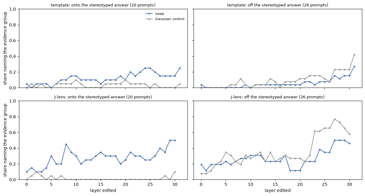
We checked that the pipeline responds to a known manipulation (subtracting directly from the stereotype token’s logit shifted the mean logit gap by an equal amount), then added controls: a random-token swap (does any added content work?), a nonce control (does any real-seeming content work?), and a Gaussian-direction swap, which acts as an approximate, leaky ablation that removes the target’s component without adding anything specific. We also used patching as a positive control.
The picture is humbling:
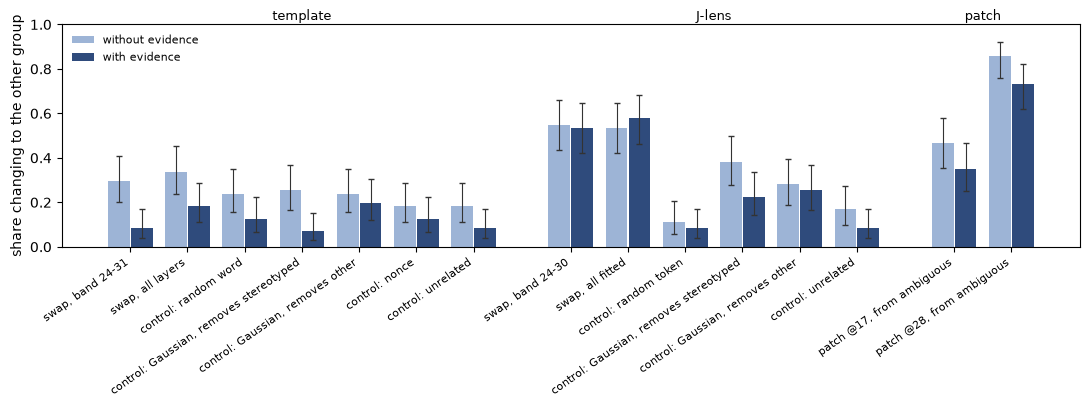
Swaps are strongest late in the network. Single-layer swaps work within the workspace band, especially layers 20–30, while interventions at layers 1–5 leave the final-layer readout unchanged. That means either this band is too early to act directly on the output, or the model recovers the concept downstream. We cannot yet say which.
Dose matters, and damage is easy. On Winogender, a he/she coordinate swap across layers 20–30 shifts the mean log p(she) − log p(he) by +1.78, +2.53, +3.18 and +4.25 nats at α = 0.5, 1, 1.5 and 2, reversing the preference in 85–96% of the 120 prompts, while frequency-matched sham and norm-matched random controls stay near zero. From about α = 2.75 the lens readout starts oscillating between source- and target-token variants, and at α ≥ 3 KL divergence spikes, held-out WikiText loss degrades, and the sham pair spuriously triggers 77.5% flips. Any effect at α ≥ 3 reflects generalized damage, not targeted axis control, so we treat α ≤ 2 as the safe range. Note too that the swap inverts a direction; it is not evidence of demographic parity.
A statistical direction is not enough. A difference-of-means direction learned from 240 paired male/female-pronoun sentences was internally consistent (pair cosine peaking at layers 26–29), yet at α = 1 it shifted preference by only +0.26 nats with 32% flips (KL = 0.058), far below the lens swap (+2.53 nats, ~96% flips). A direction that merely separates examples is a weaker handle than one built to alter output logits.
Late layers hold bias in more than one direction. Late layers appear to store the signal in a multi-dimensional subspace that one direction can reduce but not remove, and edits in middle layers can be undone downstream. In one case, ablating the single token “he” cut P(she) from 44.6% to 17.7%, which points to grammatical entanglement, while subtracting the she-minus-he difference vector moved P(she) to 7.9% and raised P(he) from 1.5% to 48.8%. Strong flips can also push activations off-distribution, so flip rate alone can overstate success.
A model can answer correctly and still hold the stereotype. That is what the J-lens lets us see: in Qwen3.5-4B, stereotype-congruent content surfaces in the workspace even when the output never states it, and even when the context has already settled the question.
The strongest case is gender, where the lens’s occupational preferences track US labor statistics and a permuted null stays flat. Step outside that setting and the signal gets slippery: in balanced datasets like BBQ, stereotyped and counter-stereotyped cases cancel, group priors absorb most of the variance, and a change of descriptor can move the readout more than a change of group. Where the signal lives is equally layered. Correlations peak around layers 23–25, layer 27 lights up both answers at once, and steering is most effective at layers 29–30. Lens directions give us a handle on the committed answer, but a swap adds little beyond ablating the answer the model was already giving, and at α ≥ 3 the output loses coherence.
The lesson is less about any single number than about method. A readout is evidence, not a verdict. Finding bias in a model’s inner workings means triangulating across lenses, controls and datasets, and testing whether the signal actually drives the answer or merely sits beside it.